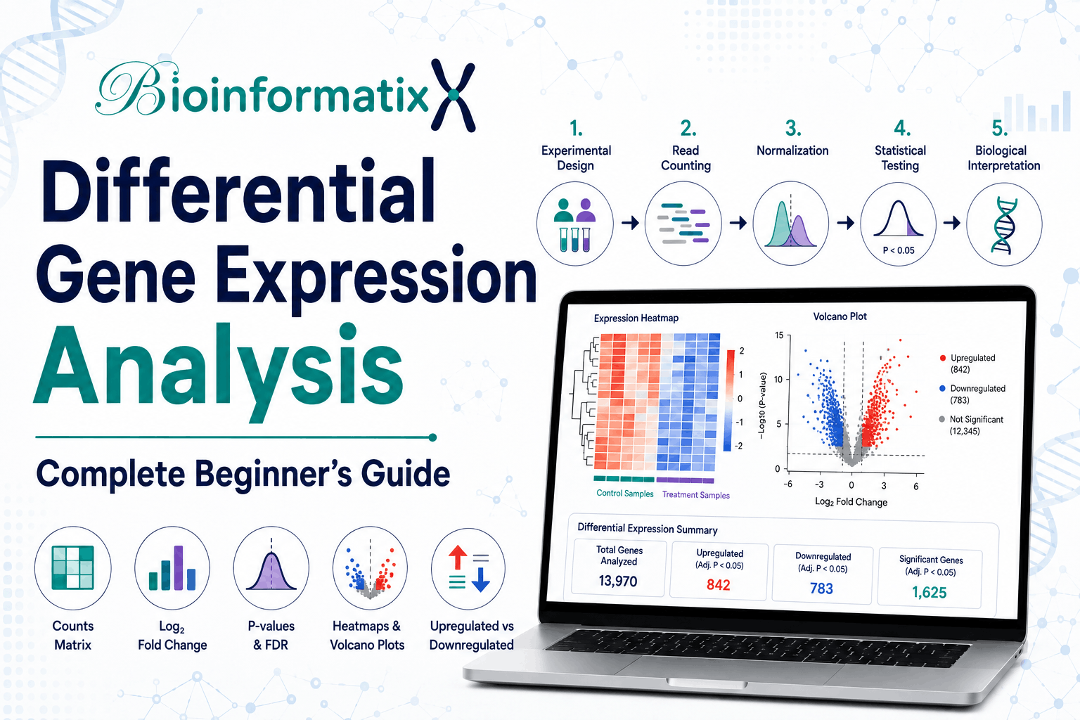
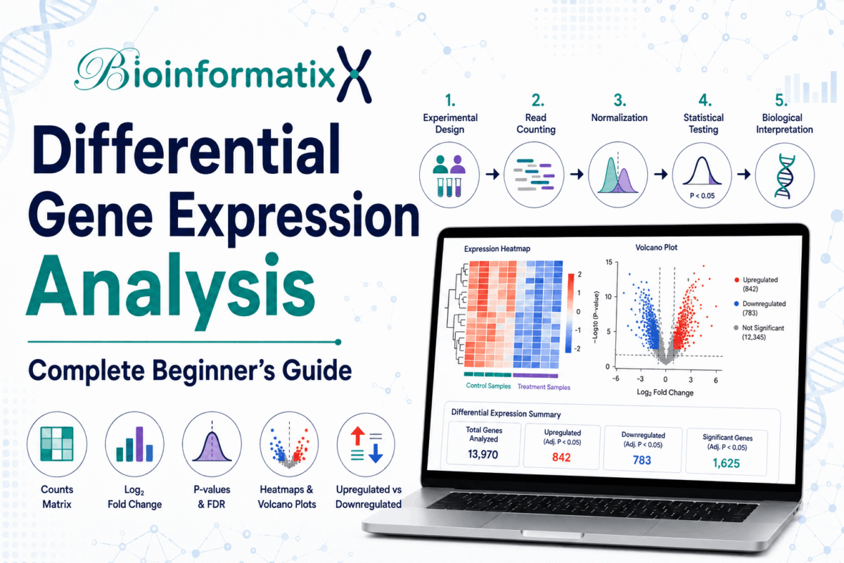
Differential Gene Expression Analysis is one of the most important computational approaches in transcriptomics. It allows researchers to identify genes whose expression levels differ systematically between biological conditions, such as disease versus healthy tissue, treated versus untreated samples, or different developmental stages.
In RNA-Seq studies, millions of sequencing reads are ultimately summarized into gene-level or transcript-level measurements. Differential Gene Expression Analysis then applies statistical methods to determine which expression differences are supported by the data rather than simply reflecting biological or technical variability.
For aspiring bioinformaticians and NGS data analysts, differential expression is an essential skill because it connects RNA sequencing with statistics, R programming, visualization, pathway analysis, biomarker discovery, and biological interpretation.
In this complete beginner’s guide, you will learn:
- What Differential Gene Expression Analysis is
- What a differentially expressed gene (DEG) means
- How RNA-Seq count matrices are generated
- Why biological replicates are essential
- Raw counts vs normalized counts vs TPM
- How normalization works
- How DESeq2, edgeR, and limma-voom are used
- What log2 fold change means
- P-values vs adjusted P-values
- How to interpret PCA, MA plots, volcano plots, and heatmaps
- How batch effects influence differential expression
- Differential expression in bulk and single-cell RNA-Seq
- How to perform functional analysis after identifying DEGs
- Common mistakes beginners should avoid
- How to learn transcriptomics and differential expression practically
If you are new to RNA sequencing, first read our RNA-Seq Explained: A Complete Beginner’s Guide to RNA Sequencing.
If you are new to sequencing more broadly, start with What Is Next-Generation Sequencing (NGS)?.
What Is Differential Gene Expression Analysis?
Differential Gene Expression Analysis is the statistical comparison of gene-expression measurements between biological conditions.
Suppose researchers collect RNA-Seq data from two groups:
Healthy Samples
vs
Cancer Samples
After sequencing and quantification, they may obtain a count matrix such as:
| Gene | Healthy 1 | Healthy 2 | Healthy 3 | Cancer 1 | Cancer 2 | Cancer 3 |
|---|---|---|---|---|---|---|
| GeneA | 120 | 133 | 115 | 890 | 825 | 910 |
| GeneB | 650 | 612 | 670 | 190 | 205 | 177 |
| GeneC | 88 | 91 | 84 | 92 | 86 | 95 |
GeneA appears to have higher expression in cancer, while GeneB appears lower.
But visual differences alone are not enough.
Differential-expression software evaluates expression differences relative to variability among biological replicates. For example, DESeq2 models RNA-Seq count data using negative-binomial generalized linear models and estimates both expression changes and biological dispersion.
The ultimate objective is to distinguish:
systematic biological differences
from:
variation expected among samples
What Is a Differentially Expressed Gene?
A differentially expressed gene, commonly abbreviated as DEG, is a gene for which statistical analysis provides evidence that expression differs between the conditions being compared.
For example:
Treatment
vs
Control
A gene could show:
higher expression in treatment → upregulated
or:
lower expression in treatment → downregulated
However, a DEG should not be defined using fold change alone.
A proper decision generally considers both:
effect size
and:
statistical evidence
This distinction is central to Differential Gene Expression Analysis.
Why Is Differential Gene Expression Analysis Important?
Many biological processes involve changes in gene activity rather than changes in the underlying DNA sequence.
Differential expression can therefore help researchers understand how biological systems respond to disease, treatment, development, environmental stress, genetic perturbation, infection, and many other conditions.
Applications include:
| Research Area | Example Question |
|---|---|
| Cancer biology | Which genes differ between tumor and normal tissue? |
| Drug research | Which genes respond to a treatment? |
| Immunology | Which pathways activate after infection? |
| Plant science | Which genes respond to drought or salinity? |
| Development | Which genes change across developmental stages? |
| Biomarker research | Which genes distinguish disease from healthy samples? |
| Neuroscience | Which transcripts differ among brain regions or conditions? |
| Microbiology | How does gene expression change under stress? |
The same statistical principles can also be adapted to more complex transcriptomics experiments.
Where Does Differential Expression Fit in the RNA-Seq Workflow?
Differential expression occurs relatively late in a standard RNA-Seq pipeline.
A typical workflow is:
Biological Samples
↓
RNA Extraction
↓
RNA-Seq Library Preparation
↓
Sequencing
↓
FASTQ
↓
Quality Control
↓
Alignment or Transcript Quantification
↓
Gene/Transcript Quantification
↓
Count Matrix
↓
Differential Gene Expression Analysis
↓
DEGs
↓
Functional Enrichment
↓
Biological Interpretation
This means differential expression does not begin directly from FASTQ reads.
The sequencing reads must first be converted into quantitative measurements for genes or transcripts.
BioInformatix covers this complete upstream workflow in the Hands-On RNA-Seq Analysis Crash Course: From FASTQ to Differential Expression. The current course moves from sequencing-data retrieval and preprocessing through alignment, quantification, differential expression, and downstream interpretation.
Step 1: Start with a Good Experimental Design
Before opening R or running DESeq2, you need an appropriate experiment.
Consider this example:
| Group | Samples |
|---|---|
| Control | Control1, Control2, Control3 |
| Treatment | Treatment1, Treatment2, Treatment3 |
Here there are three biological replicates in each condition.
Biological replication is essential because differential-expression methods need information about variability between independently sampled biological units.
Without replication, it becomes difficult or impossible to reliably estimate biological variation.
Biological Replicates vs Technical Replicates
These concepts are frequently confused.
Biological Replicates
Independent biological samples representing variability within a population.
For example:
Patient 1
Patient 2
Patient 3
Technical Replicates
Repeated measurements from the same underlying biological material.
For example:
Patient 1 sequencing run A
Patient 1 sequencing run B
Increasing technical sequencing depth is not equivalent to adding independent biological replicates.
For differential expression, experimental design should reflect the actual biological question.
Step 2: Generate an Expression Count Matrix
After RNA-Seq alignment or transcript quantification, expression values are summarized across samples.
For alignment-based analysis, a tool such as featureCounts may generate gene-level counts.
Conceptually:
FASTQ
↓
STAR / HISAT2
↓
BAM
↓
featureCounts
↓
Gene × Sample Count Matrix
A matrix may look like:
| Gene | Control1 | Control2 | Control3 | Treatment1 | Treatment2 | Treatment3 |
|---|---|---|---|---|---|---|
| GeneA | 102 | 118 | 110 | 450 | 487 | 462 |
| GeneB | 922 | 870 | 905 | 420 | 401 | 433 |
| GeneC | 12 | 9 | 14 | 11 | 13 | 10 |
For standard DESeq2 workflows, the package expects unnormalized count data or suitable estimated counts rather than expression values that have already been normalized by library size. DESeq2 internally estimates normalization factors as part of its model.
Raw Counts vs Normalized Counts vs TPM
This is one of the most important concepts in Differential Gene Expression Analysis.
Raw Counts
Raw gene counts represent the number of sequencing reads or fragments assigned to each gene according to the quantification method.
Example:
GeneA = 325 reads
GeneB = 1420 reads
GeneC = 78 reads
Count-based methods such as DESeq2 model these count measurements statistically. DESeq2 specifically expects an unnormalized count matrix, or appropriate estimated counts imported from transcript-level quantification workflows.
Normalized Counts
Sequencing libraries rarely contain exactly the same number of reads.
One sample may contain:
20 million reads
while another contains:
40 million reads
Raw counts therefore cannot always be compared directly.
Normalization adjusts for systematic differences such as sequencing depth or effective library size.
DESeq2, for example, estimates sample-specific size factors before estimating dispersion and fitting its negative-binomial model.
TPM
TPM stands for:
Transcripts Per Million
TPM incorporates gene or transcript length and sequencing depth and can be useful for describing relative expression abundance.
However, TPM values should not simply be substituted for count data when using statistical methods designed for counts.
For DESeq2 specifically, normalized expression values such as library-size-scaled counts should not be supplied in place of the expected count input.
Why Is Normalization Necessary?
Imagine two libraries:
Sample A = 10 million reads
Sample B = 30 million reads
Suppose a gene receives:
Sample A = 1,000 reads
Sample B = 2,000 reads
At first glance, Sample B appears to show twice as much expression.
But Sample B also has three times as many total sequencing reads.
This illustrates why raw counts alone cannot always be interpreted as direct expression differences.
Normalization allows statistical models to account for systematic library differences before testing biological contrasts.
Step 3: Filter Very Lowly Expressed Genes
RNA-Seq matrices often contain genes with extremely few counts.
For example:
GeneX:
0 0 1 0 0 0
Such genes generally provide little information for detecting reliable group-level expression changes.
Filtering very low-count genes can:
reduce the number of uninformative tests
and:
improve statistical efficiency
DESeq2 also performs independent filtering in its results workflow based on mean normalized counts to increase the number of detectable genes at a specified significance threshold.
The exact filtering strategy should be chosen according to the statistical workflow rather than copied blindly from an unrelated dataset.
Step 4: Prepare Sample Metadata
The expression matrix alone is not enough.
You also need metadata explaining what each sample represents.
For example:
| Sample | Condition | Batch | Sex |
|---|---|---|---|
| Control1 | Control | 1 | Female |
| Control2 | Control | 1 | Male |
| Control3 | Control | 2 | Female |
| Treatment1 | Treatment | 1 | Female |
| Treatment2 | Treatment | 1 | Male |
| Treatment3 | Treatment | 2 | Female |
This information allows the statistical model to represent the experimental design correctly.
In DESeq2, a design formula specifies which variables should be incorporated when estimating expression effects.
For example:
design = ~ condition
or a more complex experiment might use:
design = ~ batch + condition
The exact model depends on the experiment.
Batch Effects in Differential Gene Expression Analysis
A batch effect is a systematic technical difference among groups of samples.
Potential sources include:
Different sequencing runs
Different library-preparation dates
Different laboratories
Different reagent batches
Different processing times
Suppose:
All controls = Batch 1
All treatments = Batch 2
Now biological condition and batch are perfectly confounded.
If expression differs, it may be impossible to determine whether the difference was caused by treatment or batch.
DESeq2 documentation specifically notes that perfectly confounded design variables cannot be estimated separately because the model matrix becomes non-identifiable.
Good experimental design is therefore more valuable than trying to computationally repair a fundamentally confounded experiment later.
Step 5: Explore the Samples Before Statistical Testing
Before interpreting DEGs, examine how the samples relate to each other.
Common exploratory methods include:
Principal Component Analysis
sample-to-sample distance
expression distributions
library-size inspection
These checks can reveal unexpected structure before formal differential-expression testing.
PCA in Differential Gene Expression Analysis
Principal Component Analysis (PCA) reduces a high-dimensional gene-expression dataset into a small number of axes that explain major patterns of variation.
Conceptually, thousands of genes are summarized into:
PC1
PC2
PC3
...
A PCA plot can help detect:
group separation, sample outliers, batch effects, and unexpected clustering.
DESeq2 provides PCA functionality for transformed expression data as part of its recommended sample-quality assessment workflow.
For example, if biological replicates cluster closely while treatment and control separate primarily along PC1, this can be consistent with a strong condition-associated expression pattern.
However, PCA separation itself does not prove differential expression or biological causality.
Differential Gene Expression Analysis with DESeq2
DESeq2 is one of the most widely used Bioconductor packages for count-based differential-expression analysis.
The official DESeq2 Bioconductor documentation describes a workflow based on negative-binomial generalized linear models. DESeq2 estimates sample size factors, gene-specific dispersion, model coefficients, and statistical tests for specified experimental contrasts.
A simplified workflow is:
Count Matrix
+
Sample Metadata
↓
DESeqDataSet
↓
Normalization
↓
Dispersion Estimation
↓
Model Fitting
↓
Statistical Testing
↓
Differential Expression Results
DESeq2 is particularly useful because it can accommodate experimental designs more sophisticated than a simple two-group comparison.
What Is Dispersion in RNA-Seq?
Biological replicates do not produce identical gene counts.
Suppose one gene has:
Control:
100, 110, 95

Treatment:
500, 520, 490
The expression difference is large and within-group variability is relatively small.
Compare that with:
Control:
100, 500, 20

Treatment:
200, 700, 40
Although some counts differ strongly, the samples are highly variable.
Differential-expression models need to account for this variation.
DESeq2 models gene counts with a negative-binomial distribution that includes a gene-specific dispersion parameter, allowing variance to exceed the mean in biological count data.
Differential Gene Expression Analysis with edgeR
edgeR is another major Bioconductor package for differential analysis of count data.
The official edgeR documentation describes the package as supporting differential analysis of sequencing-derived read-count data, including RNA-Seq and other sequencing assays.
Like DESeq2, edgeR models count variability using negative-binomial approaches.
A conceptual edgeR workflow involves:
Counts
↓
Filtering
↓
Library normalization
↓
Dispersion estimation
↓
Model fitting
↓
Statistical testing
↓
DEGs
Both DESeq2 and edgeR are widely used, and learning the principles behind each is more useful than treating one package as universally superior.
BioInformatix’s Learn Advanced Transcriptomics: lncRNA, miRNA & Psi-Seq Data Analysis includes differential-expression analysis with DESeq2 and edgeR as part of its lncRNA workflow.
Differential Expression with limma-voom
limma is another major Bioconductor framework for gene-expression analysis.
It was originally developed extensively around microarray-style expression data, while the voom methodology enables RNA-Seq count data to be analyzed within limma’s linear-model framework by modeling the mean-variance relationship.
The official limma documentation provides the package and associated user guides, and Bioconductor maintains RNA-Seq workflows based on edgeR and limma-voom.
Therefore, common RNA-Seq differential-expression choices include:
| Method | General Approach |
|---|---|
| DESeq2 | Negative-binomial generalized linear models |
| edgeR | Negative-binomial count modeling |
| limma-voom | Mean-variance modeling + linear models |
The appropriate method depends on experimental design, data characteristics, established workflow, and research objectives.
Step 6: Understand Log2 Fold Change
Differential-expression results frequently report:
log2 fold change
or:
log2FC
Suppose a gene has twice the expression in treatment compared with control.
Then approximately:
Fold change = 2
log2(2) = +1
If expression is four times higher:
Fold change = 4
log2(4) = +2
If expression is half as high:
Fold change = 0.5
log2(0.5) = -1
Therefore:
| log2FC | Interpretation |
|---|---|
| +2 | approximately 4× higher |
| +1 | approximately 2× higher |
| 0 | no estimated change |
| -1 | approximately 2× lower |
| -2 | approximately 4× lower |
The direction depends on how the comparison is defined.
If the contrast is:
Treatment vs Control
then positive values generally indicate higher expression in treatment.
If you reverse the contrast, the sign reverses.
Always document the comparison direction.
Step 7: Understand P-Values
A statistical test evaluates whether the observed expression difference is compatible with the null model after accounting for the fitted variability.
A smaller p-value represents stronger evidence against the null hypothesis under the selected model.
However, RNA-Seq analyses often test thousands of genes simultaneously.
That creates a multiple-testing problem.
Why Adjusted P-Values Matter
Suppose you test:
20,000 genes
Even when no real biological differences exist, some genes may produce small p-values simply by chance.
Differential-expression workflows therefore use multiple-testing correction.
Results are commonly reported with an:
adjusted p-value
or:
false discovery rate-related significance measure
When interpreting DESeq2 output, the adjusted p-value is usually more relevant for selecting DEGs than the unadjusted p-value alone. DESeq2’s results workflow explicitly performs multiple-testing-aware reporting and independent filtering around an adjusted-p-value significance threshold.
How Should You Define Significant DEGs?
A commonly encountered rule might be:
Adjusted p-value < 0.05
AND
|log2FC| ≥ 1
But this should not be treated as a universal biological law.
Appropriate criteria depend on:
Study objective
Sample size
Biological system
Expected effect sizes
Statistical method
Exploratory vs confirmatory analysis
A gene with:
log2FC = 0.7
could still be biologically important.
Likewise, a gene with:
log2FC = 3
but highly uncertain statistical evidence should not automatically be considered reliable.
Report and justify your thresholds rather than choosing them only because another paper used them.
Step 8: Visualize Differential Expression Results
Differential expression becomes much easier to interpret when combined with visualization.
Several plots are particularly useful.
Volcano Plot
A volcano plot usually places:
log2 Fold Change
on the x-axis and:
-log10(p-value or adjusted p-value)
on the y-axis.
Conceptually:
           Highly significant
                 ↑

Downregulated ← 0 → Upregulated
A volcano plot makes it easy to highlight genes showing both substantial effect sizes and statistical evidence.
However, the plot itself does not determine whether a gene is biologically meaningful.
MA Plot
An MA plot visualizes expression change relative to average abundance.
Typically:
X-axis = Mean expression
Y-axis = log2 Fold Change
It can help reveal whether fold-change estimates depend strongly on expression level.
DESeq2 provides a dedicated plotMA() function for examining log2 fold changes relative to mean normalized counts.
Heatmap
A heatmap can show expression patterns across selected genes and samples.
For example:
Top Differentially Expressed Genes
↓
Transform / scale expression
↓
Cluster genes and samples
↓
Heatmap
A heatmap can reveal whether:
biological replicates cluster together
and whether:
candidate genes show coherent expression patterns
For visualization, transformed or standardized expression values are often more useful than raw counts.
PCA Plot
PCA focuses primarily on sample-level variation rather than individual genes.
Use it to investigate whether:
Control samples cluster together
Treatment samples cluster together
Batch groups dominate
Outliers are present
PCA should usually be examined before interpreting a DEG list.
Step 9: Inspect Individual Genes
A statistically significant result should also make biological sense at the sample level.
For an important candidate gene, inspect expression across individual biological replicates.
For example:
Control:
95 102 110

Treatment:
480 520 495
is much more convincing than:
Control:
20 25 500

Treatment:
50 55 600
even if summary statistics initially make both appear interesting.
DESeq2 provides functions such as plotCounts() for inspecting normalized counts of individual genes across experimental groups.
Step 10: Move from DEGs to Biological Interpretation
A spreadsheet containing 1,000 differentially expressed genes is not the final biological result.
The next question is:
What biological processes do these genes represent?
Common downstream analyses include:
Gene Ontology enrichment
Pathway enrichment
Gene Set Enrichment Analysis
Protein interaction analysis
Transcription-factor analysis
Disease association
Network analysis
For example, an RNA-Seq experiment might identify hundreds of DEGs but reveal that many belong to a smaller number of biological themes such as:
Cell cycle
Immune signaling
DNA repair
Oxidative stress
Apoptosis
Metabolism
This transition from individual genes to biological pathways is an essential part of transcriptomics.
DEG Analysis vs Gene Set Enrichment Analysis
Traditional DEG-based enrichment usually begins with a filtered list of genes.
For example:
Adjusted p-value < threshold
+
Fold-change threshold
↓
Significant gene list
↓
Pathway enrichment
Gene Set Enrichment Analysis (GSEA) instead can use a ranked gene list without requiring a hard DEG cutoff at the beginning.
This can be useful when a biological pathway changes modestly across many genes even though relatively few individual genes pass strict significance thresholds.
BioInformatix’s Learn Bioinformatics Data Analysis: Master Python, Linux and R Scripting includes differential-expression analysis and gene-set enrichment in its R-based bioinformatics training.
Differential Gene Expression Analysis in Microarray Data
Differential expression is not exclusive to RNA-Seq.
Microarray experiments also compare gene-expression measurements among conditions.
However, the underlying data differ.
| RNA-Seq | Microarray |
|---|---|
| Sequencing-derived counts | Probe-intensity measurements |
| DESeq2 / edgeR / limma-voom | Commonly limma |
| FASTQ upstream | Array intensity data upstream |
| Can support transcript discovery | Dependent on predefined probes |
Therefore, the statistical workflow should match the measurement technology.
Differential Gene Expression Analysis in Single-Cell RNA-Seq
Single-cell differential expression requires additional care.
In bulk RNA-Seq:
one sample = one expression profile
In single-cell RNA-Seq:
one biological sample
↓
thousands of cells
A common mistake is treating every cell as though it were an independent biological replicate.
Cells originating from the same biological sample are correlated. Current Seurat guidance specifically warns that treating individual cells as independent replicates can inflate false-positive findings in multi-sample differential-expression comparisons.
For replicated condition-level comparisons, a common strategy is pseudobulk analysis:
Cells
↓
Group by biological sample + cell type
↓
Sum counts
↓
Sample-level pseudobulk profiles
↓
DESeq2 / edgeR
Both current Seurat guidance and Bioconductor multi-sample single-cell workflows demonstrate sample-level pseudobulk approaches for differential-expression testing.
If you want to learn single-cell analysis practically, explore:
Learn Single-Cell RNA-Seq Data Analysis Using R and Python
BioInformatix currently positions this course around practical single-cell workflows including clustering, annotation, and differential-expression analysis.
Differential Expression in Advanced Transcriptomics
Gene-expression analysis extends beyond conventional protein-coding mRNA.
Modern transcriptomics also investigates:
lncRNAs
miRNAs
alternative transcripts
RNA modifications
other non-coding RNAs
The exact pipeline differs depending on the RNA class.
For example, lncRNA analysis may involve:
FASTQ
↓
Alignment
↓
Transcript assembly
↓
Transcript classification
↓
Quantification
↓
Differential expression
BioInformatix’s Advanced Transcriptomics course currently includes lncRNA differential-expression analysis using DESeq2 and edgeR, alongside miRNA-Seq and Ψ-seq workflows.
Public Datasets for Differential Gene Expression Analysis
You do not need to generate your own sequencing experiment to practice Differential Gene Expression Analysis.
Public datasets can be obtained through repositories such as:
NCBI GEO
and:
NCBI SRA
A practical project might follow:
Find GEO Study
↓
Read Experimental Design
↓
Identify Biological Groups
↓
Download Count Matrix
or
Download FASTQ from SRA
↓
Generate Counts
↓
Differential Gene Expression Analysis
↓
Visualization
↓
Functional Analysis
Read our GEO Database Tutorial & SRA Database Guide to learn how GSE, GSM, SRP, SRX, and SRR accessions connect public transcriptomics studies with raw sequencing data.
Processed GEO Data vs Raw RNA-Seq Reads
If a GEO study already provides a suitable count matrix, you may be able to begin relatively close to the statistical-analysis stage.
For example:
GEO Count Matrix
↓
Metadata
↓
DESeq2
If you instead retrieve raw SRA reads:
SRA
↓
FASTQ
↓
QC
↓
Alignment
↓
Quantification
↓
Count Matrix
↓
DESeq2
The second workflow gives you more control over preprocessing, reference choice, alignment, and quantification.
The first is often faster for exploratory reanalysis.
Common Differential Gene Expression Analysis Mistakes
Several mistakes can substantially weaken an otherwise technically correct transcriptomics study.
| Mistake | Why It Matters |
|---|---|
| No biological replicates | Biological variability cannot be estimated reliably |
| Using TPM directly in DESeq2 | Does not match DESeq2’s expected count model |
| Ignoring batch effects | Technical differences may be mistaken for biology |
| Mixing sample labels | Produces invalid comparisons |
| Wrong reference annotation | Gene counts may be incorrect |
| Arbitrary DEG thresholds | May exclude important effects or exaggerate weak ones |
| Using p-value instead of multiple-testing-aware results | Increases false discoveries |
| Ignoring PCA/outliers | Hidden sample problems may remain undetected |
| Choosing genes only by fold change | Ignores uncertainty |
| Stopping at the DEG list | Does not explain biological function |
| Treating single cells as independent subjects | Can inflate significance |
| Hiding unsuccessful comparisons | Reduces reproducibility |
Should You Remove an Outlier?
Suppose PCA shows one sample far away from all others.
Do not immediately delete it.
First investigate:
FASTQ quality
Mapping rate
Library size
Sample identity
Contamination
Batch information
Metadata
RNA quality
An outlier may represent:
technical failure
or:
real biological heterogeneity
Removing a sample only because it reduces statistical significance is not scientifically appropriate.
Differential Expression Does Not Prove Causation
Suppose GeneA is strongly upregulated in cancer.
Differential expression supports the statement:
GeneA expression differs between the analyzed conditions.
It does not automatically prove:
GeneA causes the cancer.
The observed change could be:
a driver
a downstream consequence
a compensatory response
associated with cell composition
associated with another confounding variable
Functional experiments and additional evidence are needed before making causal conclusions.
Is Differential Gene Expression Analysis Difficult to Learn?
The statistics can initially appear complicated, but the workflow becomes easier once you understand what each stage is doing.
A beginner should think of the process as:
Count Matrix
↓
Metadata
↓
Quality Assessment
↓
Normalization
↓
Statistical Model
↓
Contrasts
↓
DEG Results
↓
Visualization
↓
Functional Interpretation
You do not need to derive every negative-binomial equation before beginning practical RNA-Seq analysis.
But you should understand:
what the input represents
why replication matters
what normalization does
what log2FC means
why multiple testing matters
what your statistical comparison actually tests
Those concepts are much more important than memorizing R commands.
Learn Differential Gene Expression Analysis with BioInformatix
If your main objective is learning a complete bulk RNA-Seq workflow, the most directly relevant individual course is:
Hands-On RNA-Seq Analysis Crash Course: From FASTQ to Differential Expression
The course takes you beyond a prepared count table and teaches how RNA-Seq data reach the differential-expression stage through public-data retrieval, preprocessing, alignment, quantification, and downstream analysis.
This is particularly useful because understanding how counts were generated makes you a much stronger differential-expression analyst.
Learn Advanced Differential Expression in Transcriptomics
Once you understand standard RNA-Seq, continue with:
Learn Advanced Transcriptomics: lncRNA, miRNA & Psi-Seq Data Analysis
The course extends transcriptomics beyond conventional mRNA and currently includes lncRNA expression quantification and differential-expression analysis using DESeq2 and edgeR.
It is particularly relevant for researchers working with:
lncRNAs
miRNAs
RNA modifications
advanced sequencing workflows
Learn Differential Expression in Single-Cell RNA-Seq
For cell-level transcriptomics, continue with:
Learn Single-Cell RNA-Seq Data Analysis Using R and Python
The course provides a broader single-cell workflow rather than treating differential expression as an isolated statistical step.
This is important because single-cell differential analysis should be interpreted together with:
quality control
normalization
dimensionality reduction
clustering
cell-type annotation
sample identity
Become an NGS & Transcriptomics Analyst
If your goal is broader NGS expertise rather than learning Differential Gene Expression Analysis in isolation, the primary BioInformatix learning pathway is:
NGS & Transcriptomics Analyst Bundle: Master RNA-Seq, Variant Calling & Single-Cell Genomics
The BioInformatix bundle is designed as a broader pathway for students, researchers, and professionals who want practical skills across multiple modern sequencing-analysis workflows.
Instead of learning only how to generate a DEG table, the bundle helps connect differential expression with the larger NGS landscape:
NGS Fundamentals
↓
RNA-Seq
↓
Differential Gene Expression
↓
Advanced Transcriptomics
↓
Single-Cell Genomics
↓
Genomic Variant Analysis
This broader perspective is particularly useful for someone aiming to work as an NGS Data Analyst, where projects may involve several different sequencing modalities rather than one RNA-Seq comparison.
Recommended Differential Gene Expression Learning Roadmap
| Stage | What to Learn | BioInformatix Resource |
|---|---|---|
| 1 | NGS fundamentals | What Is Next-Generation Sequencing? |
| 2 | RNA sequencing concepts | RNA-Seq Explained |
| 3 | Linux fundamentals | Linux Command Line Essentials |
| 4 | Public dataset retrieval | GEO & SRA Database Guide |
| 5 | FASTQ-to-count workflow | Hands-On RNA-Seq Analysis |
| 6 | DESeq2 and DEG interpretation | Hands-On RNA-Seq Analysis |
| 7 | lncRNA and advanced transcriptomics | Advanced Transcriptomics |
| 8 | Single-cell differential expression | Single-Cell RNA-Seq |
| 9 | Broader NGS expertise | NGS & Transcriptomics Analyst Bundle |
Frequently Asked Questions
What is Differential Gene Expression Analysis?
Differential Gene Expression Analysis is a statistical approach used to identify genes whose expression differs between biological conditions.
What is a DEG?
DEG stands for differentially expressed gene.
It is a gene for which the analysis provides evidence of an expression difference between the groups being compared.
Is differential gene expression the same as RNA-Seq?
No.
RNA-Seq is the sequencing technology and workflow used to measure RNA.
Differential expression is one downstream analysis that can be performed on quantified expression data.
What data do I need for DESeq2?
DESeq2 is designed to work with an unnormalized count matrix or suitable estimated counts together with sample metadata describing the experimental design.
Can I use TPM values in DESeq2?
You should not simply use TPM or other pre-normalized abundance values as substitutes for the count input expected by the DESeq2 statistical model.
What is log2 fold change?
Log2 fold change describes the magnitude and direction of an expression difference on a logarithmic scale.
For example:
log2FC = +1
corresponds approximately to a twofold increase.
What does a negative log2 fold change mean?
For a comparison defined as treatment versus control, a negative log2FC generally means estimated expression is lower in treatment than control.
Always verify the contrast direction.
What is an adjusted p-value?
An adjusted p-value accounts for the fact that thousands of genes are tested simultaneously.
It is generally more appropriate than using unadjusted p-values alone to select DEGs in large-scale expression studies.
Is adjusted p-value < 0.05 always required?
No universal threshold is appropriate for every experiment.
The cutoff should match the study design, analytical objective, statistical method, and tolerance for false discoveries.
What is DESeq2?
DESeq2 is a Bioconductor package that models count-based expression data using negative-binomial generalized linear models for differential analysis.
What is edgeR?
edgeR is a Bioconductor package for differential analysis of sequencing count data, including RNA-Seq datasets.
What is limma-voom?
limma-voom combines RNA-Seq mean-variance modeling with the limma linear-model framework for differential-expression analysis.
What is a volcano plot?
A volcano plot visualizes expression effect size against statistical significance and is frequently used to highlight candidate DEGs.
What is an MA plot?
An MA plot displays expression change relative to average gene abundance.
What is PCA used for?
PCA helps examine major patterns of sample-level variation and can reveal clustering, outliers, or potential batch effects.
How many biological replicates do I need?
There is no single number that is optimal for every experiment. Statistical power depends on biological variability, effect size, sequencing design, and study objective. Differential-expression studies should include genuine biological replication rather than relying only on technical replicates.
Can I perform differential expression on single-cell RNA-Seq?
Yes, but replicated multi-sample comparisons require careful treatment of biological replication. Pseudobulk approaches that aggregate cells by sample and cell type are widely used to avoid treating thousands of correlated cells from one sample as independent subjects.
What should I do after identifying DEGs?
Downstream analysis may include pathway enrichment, Gene Ontology analysis, GSEA, interaction networks, literature review, candidate-gene validation, and biological interpretation.
Final Thoughts
Differential Gene Expression Analysis is one of the fundamental skills of modern transcriptomics.
The core workflow can be summarized as:
RNA-Seq
↓
Gene Counts
↓
Sample Metadata
↓
Quality Assessment
↓
Normalization
↓
Statistical Modeling
↓
log2 Fold Changes + Adjusted P-Values
↓
Differentially Expressed Genes
↓
Visualization
↓
Functional Analysis
↓
Biological Interpretation
The most important lesson is that differential expression is not simply:
high count vs low count
Reliable analysis requires you to understand biological replication, experimental design, normalization, variability, statistical testing, multiple-testing correction, effect size, and biological context.
If your immediate goal is to master the complete bulk workflow from sequencing reads to DEGs, begin with the Hands-On RNA-Seq Analysis Crash Course.
Once you understand standard RNA-Seq, progress to the Advanced Transcriptomics course for lncRNA, miRNA, and RNA-modification workflows and the Single-Cell RNA-Seq course for cell-resolved transcriptomics.
For learners who want a broader career-oriented pathway across multiple sequencing technologies, the NGS & Transcriptomics Analyst Bundle should remain the main learning destination.