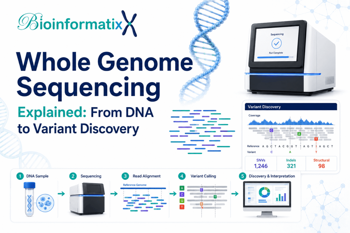
Whole Genome Sequencing (WGS) is one of the most comprehensive applications of next-generation sequencing. Rather than examining only selected genes or protein-coding regions, whole genome sequencing is designed to analyze nearly the entire genome, giving researchers access to genetic variation across coding, non-coding, regulatory and intergenic regions.
For bioinformaticians, Whole Genome Sequencing is particularly important because a WGS project brings together many fundamental NGS skills: FASTQ quality control, reference-genome preparation, read alignment, SAM/BAM processing, variant calling, VCF filtering, variant annotation and biological interpretation.
WGS can also take a different path. When an appropriate reference genome does not exist, sequencing reads can instead be reconstructed through de novo genome assembly and subsequently annotated.
In this complete beginner’s guide, you will learn:
- What Whole Genome Sequencing is
- How WGS works
- WGS vs whole-exome sequencing
- Short-read vs long-read WGS
- Sequencing depth and coverage
- Reference-based vs de novo analysis
- The complete FASTQ-to-VCF workflow
- BWA alignment
- SAM and BAM processing
- Germline and somatic variant calling
- SNPs, indels, CNVs and structural variants
- VCF files
- Variant annotation
- Genome assembly and annotation
- Important WGS bioinformatics tools
- Common beginner mistakes
- How to start learning WGS data analysis
If you are completely new to sequencing, first read our What Is Next-Generation Sequencing (NGS)? Complete Beginner’s Guide.
The U.S. National Human Genome Research Institute provides additional background on DNA sequencing and genomic research. DNA sequencing determines the order of nucleotide bases, while whole-genome approaches apply sequencing at genome scale. (Genome.gov)
What Is Whole Genome Sequencing?
Whole Genome Sequencing is an approach intended to determine sequence information across most of an organism’s genome.
For humans, that means investigating genomic information across the nuclear chromosomes as well as mitochondrial DNA, depending on the library preparation and analysis design. A genome encompasses an organism’s complete set of DNA instructions. (Genome.gov)
Unlike targeted sequencing, which examines predetermined genomic regions, WGS can provide information from:
- Protein-coding genes
- Introns
- Intergenic regions
- Promoters
- Regulatory regions
- Repetitive sequences
- Mitochondrial DNA
- Structural genomic regions
This broad genomic coverage makes Whole Genome Sequencing valuable for both research and discovery-oriented analyses.
Why Is Whole Genome Sequencing Important?
Genes occupy only part of a genome. Important biological variation can also occur outside protein-coding regions.
Whole Genome Sequencing allows researchers to investigate a much broader range of genomic variation than approaches restricted to specific genes or exons.
WGS is used in areas such as:
- Rare disease genomics
- Cancer genomics
- Population genetics
- Microbial genomics
- Infectious disease surveillance
- Pharmacogenomics
- Agricultural genomics
- Evolutionary biology
- Structural variant research
- Precision medicine
- Genome assembly
Researchers may use WGS to ask questions such as:
- Which variants are present in this genome?
- Which variants could explain a genetic phenotype?
- Which mutations arose in a tumor?
- Are large deletions or duplications present?
- How genetically related are different microbial isolates?
- Which genomic variants distinguish populations?
- Can we construct a genome for a species without a suitable reference?
WGS is considered a comprehensive genome-analysis approach and can support inherited-disease, cancer and pathogen investigations. (Illumina)
Whole Genome Sequencing vs Whole Exome Sequencing
One of the most important distinctions for beginners is WGS vs WES.
Whole Genome Sequencing
WGS attempts to sequence the genome broadly, including both coding and non-coding regions.
Whole Exome Sequencing
Whole-exome sequencing, or WES, enriches primarily for exons—the protein-coding portions of genes.
| Feature | Whole Genome Sequencing | Whole Exome Sequencing |
|---|---|---|
| Genomic scope | Broad | Mainly coding exons |
| Coding variants | Yes | Yes |
| Non-coding variants | Yes | Limited |
| Structural variant potential | Broader | More limited |
| Data volume | Larger | Smaller |
| Computational requirements | Higher | Lower |
| Target-capture step | Usually no | Yes |
| Discovery scope | Genome-wide | Coding-focused |
WES requires additional laboratory enrichment but sequences substantially less DNA than WGS, which can reduce sequencing requirements. (Genome.gov)
Neither method is automatically better.
The choice depends on:
- Research question
- Disease model
- Budget
- Number of samples
- Required genomic regions
- Variant classes of interest
- Available computational resources
Whole Genome Sequencing vs Targeted Gene Panels
Targeted sequencing focuses on a predefined collection of genes or genomic regions.
For example:
Cancer Panel → 100 Selected Genes
This can be useful when the disease genes are already well established.
Whole Genome Sequencing instead asks a broader question:
What variation exists throughout this genome?
That makes WGS especially useful for discovery-oriented analyses where the responsible genomic region may not already be known.
How Does Whole Genome Sequencing Work?
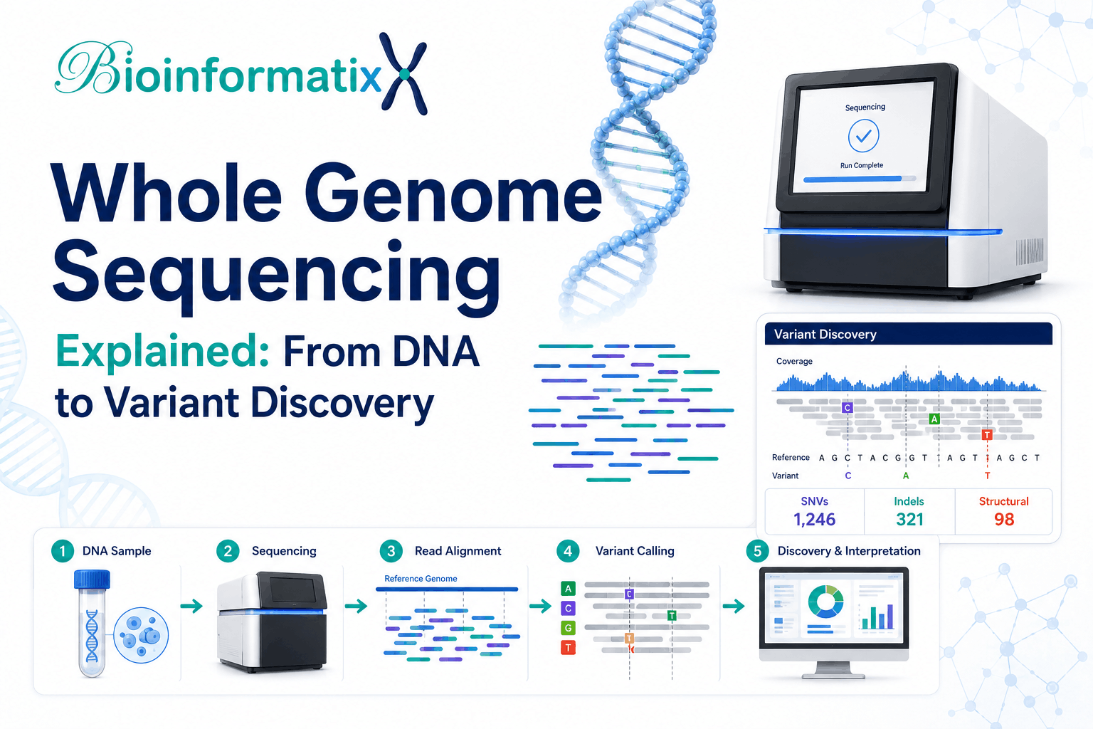
A simplified Whole Genome Sequencing workflow looks like this:
Biological Sample
↓
DNA Extraction
↓
DNA Quality Assessment
↓
Library Preparation
↓
Sequencing
↓
FASTQ Files
↓
Bioinformatics Analysis
↓
Variant Discovery or Genome Assembly
↓
Biological Interpretation
The first stages take place in the laboratory.
The later stages are where bioinformatics becomes essential.
Step 1: Biological Sample and DNA Extraction
Whole Genome Sequencing can begin with DNA extracted from many sample types, including:
- Blood
- Saliva
- Tumor tissue
- Cultured cells
- Microbial isolates
- Plant tissue
- Environmental organisms
High-quality DNA is required for reliable sequencing.
The exact DNA-quality requirements depend on the sequencing technology. Long-read sequencing, for example, often benefits from high-molecular-weight DNA because longer intact molecules enable longer reads.
Step 2: Library Preparation
DNA must be converted into a sequencing-compatible library.
Depending on the platform and workflow, library preparation may include:
- DNA fragmentation
- End repair
- Adapter ligation
- PCR amplification
- Sample indexing
- Size selection
Indexes or barcodes make it possible to sequence multiple samples together and separate their reads computationally afterward.
Step 3: Sequencing the Genome
Modern WGS can be performed using either short-read or long-read technologies.
The chosen platform affects:
- Read length
- Error characteristics
- Throughput
- Required depth
- Structural-variant detection
- Genome assembly
- Computational workflow
Short-Read Whole Genome Sequencing
Short-read sequencing generates millions or billions of relatively short reads.
A paired-end experiment usually produces files such as:
Patient01_R1.fastq.gz
Patient01_R2.fastq.gz
Short-read WGS is widely used for:
- SNP detection
- Small indel calling
- Germline genomics
- Cancer genomics
- Population genetics
- Microbial genomics
It benefits from a mature ecosystem of alignment and variant-calling tools.
Long-Read Whole Genome Sequencing
Long-read technologies generate much longer DNA reads.
Long reads are especially useful for:
- Structural variants
- Repetitive regions
- Complex rearrangements
- Haplotyping
- De novo genome assembly
- Large insertions and deletions
Short and long reads can also be combined in hybrid sequencing workflows.
Whole Genome Sequencing Coverage Explained
One of the most important concepts in WGS is coverage.
Two related metrics are commonly discussed:
- Depth of coverage
- Breadth of coverage
What Is Sequencing Depth?
Sequencing depth describes approximately how many reads cover a genomic position.
For example:
30× coverage
means that a position is represented by roughly 30 sequencing observations on average.
A simplified estimate is:
Average coverage =
Total sequenced bases / Genome size
For a 3-gigabase genome:
90 Gb sequencing data
÷
3 Gb genome
≈
30× average coverage
NHGRI similarly describes sequence coverage as an important consideration when estimating genome-sequencing requirements. (Genome.gov)
What Is Breadth of Coverage?
Breadth describes the proportion of the genome that achieves a specified amount of sequencing coverage.
A sample could theoretically have good average sequencing depth while still containing poorly covered genomic regions.
This can occur because of:
- GC bias
- Repetitive DNA
- Library-preparation bias
- Mapping ambiguity
- Sequencing limitations
Therefore:
Average depth ≠ perfect coverage of every genomic base.
Two Major Whole Genome Sequencing Analysis Strategies
Once sequencing is complete, WGS analysis typically follows one of two broad strategies.
1. Reference-Based Whole Genome Sequencing
If a high-quality reference genome exists, reads can be aligned against it.
The workflow is:
FASTQ
↓
Reference Genome
↓
Alignment
↓
BAM
↓
Variant Calling
↓
VCF
↓
Variant Annotation
This is common in:
- Human genomics
- Clinical research
- Population genetics
- Cancer studies
2. De Novo Genome Assembly
When no suitable reference genome exists—or when reconstructing the genome itself is the scientific objective—the reads can be assembled.
The workflow becomes:
FASTQ
↓
Quality Control
↓
Genome Assembly
↓
Contigs
↓
Scaffolds
↓
Assembly Quality Assessment
↓
Genome Annotation
This is common in:
- Microbial genomics
- Non-model organisms
- New reference genomes
- Plant genomics
- Comparative genomics
These two branches explain why variant calling and genome assembly are both major WGS bioinformatics skills.
Complete Reference-Based Whole Genome Sequencing Workflow
A standard short-read WGS variant-discovery pipeline can be summarized as:
FASTQ
↓
Quality Control
↓
Read Preprocessing
↓
Reference Genome Preparation
↓
Alignment
↓
SAM/BAM
↓
Sorting & Indexing
↓
Alignment QC
↓
Variant Calling
↓
VCF
↓
Variant Filtering
↓
Variant Annotation
↓
Variant Prioritization
↓
Biological Interpretation
Let’s examine each stage.
Step 1: Obtain the FASTQ Files
FASTQ is usually the starting file format for sequencing analysis.
For paired-end sequencing:
Sample01_R1.fastq.gz
Sample01_R2.fastq.gz
Each FASTQ record contains:
- Read identifier
- DNA sequence
- Separator
- Base-quality scores
Public WGS data can also be downloaded from the NCBI Sequence Read Archive.
The official SRA Toolkit supports tools such as prefetch and fasterq-dump for retrieving public sequencing runs and converting them to FASTQ. (NCBI)
For a step-by-step explanation, read our:
GEO Database Tutorial & SRA Database Guide
Step 2: Perform FASTQ Quality Control
Before alignment, evaluate the raw sequencing reads.
Common quality metrics include:
- Per-base quality
- GC content
- Adapter contamination
- Read length
- Duplication
- Overrepresented sequences
Popular tools include:
- FastQC
- MultiQC
- fastp
A typical workflow is:
FASTQ → FastQC → Evaluate Results → Decide Whether Preprocessing Is Required
Do not trim sequencing reads simply because a tutorial says to do so.
Quality-control results should guide preprocessing decisions.
Step 3: Trim and Filter Reads When Necessary
Potential preprocessing operations include:
- Adapter removal
- Quality trimming
- Very short read removal
- Technical contaminant filtering
Common tools include:
- fastp
- Cutadapt
- Trimmomatic
After preprocessing, it is good practice to reassess read quality.
Step 4: Select the Correct Reference Genome
A reference-based WGS pipeline requires an appropriate reference genome.
The reference is normally provided as FASTA:
reference.fa
For human sequencing, genome assembly is particularly important.
Examples include:
- GRCh37
- GRCh38
Do not directly mix:
GRCh38-aligned sequencing data
with:
GRCh37 annotations or coordinates
Genome assembly consistency should be maintained across:
- Reference FASTA
- BAM files
- VCF files
- BED files
- Gene annotation
- Variant databases
Our Ensembl Genome Browser Guide explains genome assemblies, genomic coordinates and transcript annotation in more detail.
Step 5: Align Whole Genome Sequencing Reads
Short WGS reads are commonly aligned against the reference genome.
One important aligner is BWA.
Conceptually:
FASTQ + Reference FASTA
↓
Read Alignment
↓
SAM/BAM
The aligner attempts to determine where each sequence read originated in the reference genome.
A dedicated article in this NGS cluster will cover:
BWA Tutorial: Read Alignment for Whole Genome Sequencing
What Is Mapping Quality?
A read may align uniquely to one genomic location, or it may align equally well to several locations.
Mapping quality represents confidence in the chosen alignment.
Low mapping confidence can occur in:
- Repetitive DNA
- Duplicated genes
- Highly homologous regions
- Low-quality reads
- Short sequences
- Structurally complex regions
This matters because inaccurate alignment can produce false-positive or missed variant calls.
Step 6: SAM and BAM Processing
Aligned sequencing reads are commonly stored in SAM, BAM or CRAM formats.
SAM
SAM stands for Sequence Alignment/Map and is text based.
BAM
BAM is the binary representation of SAM.
CRAM
CRAM is another compressed format designed for efficient alignment storage.
The official HTS specifications define SAM and BAM as alignment formats, with BAM serving as the binary equivalent of SAM. (samtools.github.io)
A common workflow is:
SAM
↓
BAM
↓
Sorted BAM
↓
Indexed BAM
SAMtools in Whole Genome Sequencing
SAMtools is commonly used for operations such as:
- Viewing alignments
- Converting alignment formats
- Sorting BAM
- Indexing BAM
- Filtering alignments
- Extracting regions
- Calculating statistics
BAM indexing also supports efficient access to specific genomic regions. (samtools.github.io)
Step 7: Evaluate Alignment Quality
Before variant calling, evaluate the aligned reads.
Important metrics include:
- Total reads
- Mapped reads
- Mapping percentage
- Properly paired reads
- Duplicate rate
- Mapping quality
- Coverage depth
- Coverage breadth
- Insert-size distribution
Poor alignment results may indicate:
- Incorrect reference genome
- Sample contamination
- Low sequence quality
- Unexpected organism
- Sequencing problems
Do not blindly proceed to variant calling when the upstream alignment is poor.
Step 8: Duplicate Handling
Sequencing libraries can contain duplicate reads.
Depending on the workflow, duplicates may be:
- Marked
- Removed
- Retained but ignored by downstream tools
Duplicate handling is especially relevant for PCR-amplified libraries because repeated observations arising from amplification do not necessarily represent independent DNA fragments.
The appropriate strategy depends on the library protocol and analytical pipeline.
Whole Genome Sequencing Variant Calling
One of the most important applications of Whole Genome Sequencing is identifying differences between the sample and reference genome.
This is called variant calling.
Common variant-analysis tools include:
- GATK
- BCFtools
- FreeBayes
- DeepVariant
The GATK HaplotypeCaller can identify SNPs and small indels and performs local haplotype reassembly in candidate variant regions. (GATK)
If your main goal is to learn this workflow practically, the most relevant BioInformatix course is:
Learn Variant Calling NGS Data Analysis: A Hands-on Bioinformatics Course
The current BioInformatix course focuses specifically on NGS variant analysis, including alignment and variant-detection workflows. (bioinformatix.co)
Types of Genetic Variants Detected from WGS
Whole Genome Sequencing can support detection of several classes of variation.
Single Nucleotide Variants
A single base differs from the reference:
Reference: A
Sample:    G
This is a single nucleotide variant, or SNV.
Insertions
An insertion adds sequence relative to the reference.
For example:
Reference: ACCTG
Sample:    ACCAATG
Deletions
A deletion removes sequence relative to the reference.
For example:
Reference: ACCAATG
Sample:    ACCTG
Small insertions and deletions are collectively called:
indels
Structural Variants
Structural variants involve larger genomic changes, such as:
- Large deletions
- Insertions
- Duplications
- Inversions
- Translocations
- Complex rearrangements
Long-read WGS can be particularly valuable for resolving some structurally complex regions.
Copy Number Variants
Copy number variants involve changes in the number of copies of a genomic region.
For example:
Expected:
2 copies

Sample:
1 copy
or:
Sample:
4 copies
CNVs can be relevant to:
- Genetic disorders
- Cancer
- Genome evolution
- Population diversity
Germline vs Somatic Variant Calling
Variant-calling workflows also differ according to the biological question.
Germline Variant Calling
Germline variants are variants present in an individual’s inherited or constitutional genome.
Applications include:
- Rare disease genomics
- Mendelian genetics
- Population genomics
- Pharmacogenomics
A germline workflow might look like:
Patient FASTQ
↓
Alignment
↓
BAM
↓
Germline Variant Calling
↓
VCF
↓
Annotation
↓
Candidate Variant Prioritization
Somatic Variant Calling
Somatic variants arise during an individual’s lifetime and are particularly important in cancer.
A common design is:
Tumor
vs
Matched Normal
The goal is to identify mutations present in the tumor that are not part of the patient’s normal constitutional genome.
Somatic analysis can be complicated by:
- Tumor purity
- Normal-cell contamination
- Subclonal mutations
- Copy-number changes
- Heterogeneous tumor populations
Somatic and germline variant calling should therefore not be treated as identical pipelines.
What Is a VCF File?
Variant-calling results are commonly stored in VCF, or Variant Call Format.
A simplified example is:
#CHROM   POS       ID   REF   ALT   QUAL
1        123456    .    A     G     99
VCF can store information such as:
- Chromosome
- Position
- Variant ID
- Reference allele
- Alternative allele
- Quality
- Filter status
- Variant annotations
- Genotypes
- Read depth
VCF and its binary counterpart BCF are standardized genomic variant formats used throughout modern genomics workflows. (samtools.github.io)
Variant Filtering
Variant callers intentionally attempt to detect candidate variants.
Not every candidate should automatically be considered reliable.
Variant filtering may evaluate:
- Variant quality
- Read depth
- Mapping quality
- Allele balance
- Strand-related metrics
- Caller-specific annotations
The correct filters depend on:
- Sequencing technology
- Variant caller
- Study design
- Variant class
- Germline vs somatic analysis
Avoid copying filtering thresholds from an unrelated tutorial without understanding them.
Variant Annotation After Whole Genome Sequencing
A raw genomic variant alone tells you relatively little.
For example:
chr11:12345678 A>G
Variant annotation connects genomic coordinates with biological information such as:
- Gene
- Transcript
- Exon or intron
- Protein change
- Functional consequence
- Population frequency
- Existing variant identifier
One widely used resource is the official Ensembl Variant Effect Predictor (VEP).
VEP can predict consequences of SNPs, insertions, deletions, CNVs and structural variants on genes, transcripts and protein sequences. (Ensembl)
Common predicted consequences include:
- Missense variant
- Synonymous variant
- Stop-gained variant
- Frameshift variant
- Splice-site variant
- Intronic variant
- UTR variant
- Intergenic variant
Why Transcript Selection Matters
A genomic variant does not always have one consequence.
The same variant can be:
Missense in Transcript A
but:
Intronic in Transcript B
For reproducible analysis, record:
- Genome assembly
- Gene ID
- Transcript ID
- Transcript version
- Genomic position
- Reference allele
- Alternative allele
Our Ensembl Genome Browser Guide explains transcripts, MANE, Ensembl identifiers and variant consequences in greater detail.
Variant Calling vs Variant Interpretation
These two terms are frequently confused.
Variant Calling
Answers:
Where does this genome differ from the reference?
Variant Annotation
Answers:
Which genes, transcripts or genomic features overlap those variants?
Variant Interpretation
Asks:
What biological or clinical importance might these variants have?
A technically correct variant caller does not automatically produce a biological diagnosis.
Variant Prioritization
A human whole-genome analysis may produce a very large number of candidate variants.
Researchers therefore progressively prioritize them.
A simplified rare-disease workflow might look like:
Raw Variants
↓
Quality Filtering
↓
Population Frequency
↓
Functional Consequence
↓
Inheritance Pattern
↓
Gene/Disease Relationship
↓
Phenotype Compatibility
↓
Candidate Variants
The precise filtering strategy depends on the research question.
Whole Genome Sequencing and De Novo Genome Assembly
Variant calling is not the only application of WGS.
When an organism does not have a suitable reference—or when the goal is to create a genome assembly—the sequence reads can instead be assembled.
A typical workflow is:
FASTQ
↓
Quality Control
↓
Assembly
↓
Contigs
↓
Scaffolds
↓
Assembly Assessment
↓
Genome Annotation
This is especially important in microbial, plant and non-model organism genomics.
What Is a Contig?
A contig is a continuous sequence reconstructed from overlapping sequencing reads.
Conceptually:
Read 1   ─────────
Read 2       ─────────
Read 3            ─────────
                 ↓
Contig   ───────────────────
A draft genome may contain hundreds or thousands of contigs.
What Is a Scaffold?
A scaffold represents a larger ordered structure that can contain multiple contigs connected with information about their relative position or orientation.
Conceptually:
Contig 1 ---- gap ---- Contig 2
Common Genome Assembly Tools
Assemblers vary according to sequencing technology.
Examples include:
Short-Read Assembly
- SPAdes
Long-Read Assembly
- Flye
- Canu
Assembly Assessment
- QUAST
Genome assembly requires more than simply producing long contigs. Quality should be evaluated using multiple metrics and, where possible, biological completeness assessments.
Genome Annotation
Once a genome has been assembled, researchers need to identify biological features.
Genome annotation can include:
- Protein-coding genes
- rRNA
- tRNA
- Repetitive regions
- Functional annotations
For learners interested in this alternative WGS branch, BioInformatix offers:
Learn Genome Assembly and Annotation in Prokaryotes and Eukaryotes
The course is currently listed within BioInformatix’s Genomics & NGS Analysis category and focuses on genome assembly and annotation workflows. (bioinformatix.co)
Whole Genome Sequencing in Rare Disease Research
Whole Genome Sequencing can provide access to genomic regions not routinely covered by exome sequencing.
Depending on data quality and analysis methods, researchers may investigate:
- Coding variants
- Splice-related variants
- Deep intronic variants
- Regulatory variation
- Structural variants
- Copy-number variants
The broader genomic scope also means substantially more data must be filtered and interpreted.
WGS is increasingly important in molecular genetic investigation of rare and undiagnosed disease. (PubMed Central (PMC))
Whole Genome Sequencing in Cancer Research
Cancer genomes accumulate somatic alterations.
Whole Genome Sequencing can contribute to the investigation of:
- SNVs
- Indels
- Copy-number changes
- Structural variants
- Chromosomal rearrangements
WGS can also be integrated with:
- RNA-Seq
- Epigenomics
- Single-cell genomics
This highlights an important point: modern NGS analysis increasingly involves integration across multiple sequencing technologies.
Whole Genome Sequencing in Microbiology
Microbial WGS is widely used to study:
- Bacterial strain diversity
- Antimicrobial resistance
- Virulence
- Outbreak relationships
- Genome evolution
- Plasmids
- Comparative genomics
A microbial workflow may look like:
FASTQ
↓
Quality Control
↓
Genome Assembly
↓
Assembly QC
↓
Genome Annotation
↓
AMR/Virulence Analysis
↓
Comparative Genomics
For microbial genomics, you can also explore:
Learn Antimicrobial Resistance Detection Analysis Using Linux
Whole Genome Sequencing in Plant Genomics
Plant researchers use WGS for:
- Genome assembly
- SNP discovery
- Breeding research
- Population genomics
- Structural variation
- Comparative genomics
- Crop improvement
Large or highly repetitive plant genomes can present significant computational and assembly challenges.
Important Whole Genome Sequencing Bioinformatics Tools
A WGS analyst may encounter tools from several stages of the workflow.
Quality Control
- FastQC
- MultiQC
- fastp
Alignment
- BWA
Alignment Processing
- SAMtools
Variant Calling
- GATK
- BCFtools
- FreeBayes
- DeepVariant
Variant Annotation
- Ensembl VEP
- SnpEff
Genome Assembly
- SPAdes
- Flye
- Canu
Assembly Assessment
- QUAST
Visualization
- IGV
You do not need to learn every program simultaneously.
A better approach is to master one complete pipeline first.
Why Linux Is Important for Whole Genome Sequencing
WGS datasets can be very large, and many genomics programs are designed for Linux and command-line environments.
Linux skills are useful for:
- Managing FASTQ files
- Downloading reference genomes
- Running aligners
- Sorting BAM files
- Calling variants
- Processing VCF files
- Managing large datasets
- Running analyses on servers or HPC clusters
If Linux is new to you, start with the free:
Linux Command Line Essentials for Bioinformatics
You can also read our Linux for Bioinformatics Beginner’s Guide.
Python and R for Whole Genome Sequencing
Command-line tools perform many core WGS tasks, but programming is extremely useful for downstream analysis.
Python
Python can help with:
- Metadata processing
- VCF parsing
- Variant filtering
- Pipeline automation
- File manipulation
- Data integration
Read our Python for Bioinformatics Guide.
R
R is useful for:
- Statistical genetics
- Variant visualization
- Population genomics
- Genomic summaries
- Publication-quality figures
Read our R Programming for Bioinformatics Guide.
For structured programming training, explore:
Learn Bioinformatics Data Analysis: Master Python, Linux and R Scripting
Public Whole Genome Sequencing Data for Practice
You do not need to generate sequencing data yourself to learn WGS bioinformatics.
Public datasets can be found through resources such as:
- NCBI SRA
- BioProject
- ENA
A useful student project might involve:
- Select a public WGS study.
- Read the associated publication.
- Review sample metadata.
- Identify SRR accessions.
- Download FASTQ files.
- Run quality control.
- Align reads to the reference genome.
- Process BAM files.
- Call variants.
- Generate a filtered VCF.
- Annotate the variants.
- Interpret candidate variants.
Read our GEO Database Tutorial & SRA Database Guide before working with public sequencing datasets.
Common Whole Genome Sequencing Mistakes
Using the Wrong Reference Genome
Always verify the:
- Species
- Assembly
- Reference version
Every downstream coordinate depends on the reference used.
Mixing Genome Assemblies
Do not combine GRCh37 and GRCh38 resources as though their genomic positions are identical.
Skipping FASTQ Quality Control
Poor reads can affect mapping and downstream variant detection.
Losing Paired-End Relationships
Keep corresponding R1 and R2 FASTQ files correctly paired.
Ignoring Sample Metadata
Maintain a metadata sheet containing:
- Sample ID
- FASTQ files
- Sequencing run
- Experimental group
- Reference genome
- Library information
Calling Variants from Poor Alignments
Variant calling cannot repair a fundamentally incorrect alignment.
Inspect BAM quality first.
Treating Every VCF Entry as a Confirmed Variant
A raw variant call set still requires quality assessment and appropriate filtering.
Confusing Variant Calling with Variant Interpretation
Detecting a difference from the reference does not establish biological significance.
Ignoring Sequencing Coverage
Low-coverage genomic regions may have reduced confidence for genotype determination.
Using Arbitrary Variant Filters
Understand what every threshold measures before applying it.
Assuming WGS Perfectly Resolves the Entire Genome
Some regions remain difficult because of:
- Repetitive DNA
- Segmental duplications
- Mapping ambiguity
- GC extremes
- Complex structural variation
Whole Genome Sequencing is genome-wide, but it is not automatically error-free or uniformly informative at every base.
Is Whole Genome Sequencing Difficult to Learn?
WGS bioinformatics can look complicated because several technologies are combined in one pipeline:
- Next-generation sequencing
- Linux
- Reference genomes
- Sequence alignment
- BAM processing
- Genetic variation
- Variant calling
- Annotation
- Biological interpretation
The easiest way to learn is sequentially.
Start with:
FASTQ
↓
Quality Control
↓
BWA Alignment
↓
SAM/BAM
↓
Variant Calling
↓
VCF
↓
Variant Annotation
Once you understand that workflow, you can move into more specialized analysis such as:
- Germline genomics
- Somatic variants
- Structural variants
- Genome assembly
- Population genomics
Learn Whole Genome Variant Calling with BioInformatix
If your main goal is to analyze genomic variants from NGS data, start with:
Learn Variant Calling NGS Data Analysis: A Hands-on Bioinformatics Course
The course is directly aligned with the WGS analysis path because it teaches practical genomic variant-analysis workflows. (bioinformatix.co)
It is particularly relevant for learners interested in:
- NGS variant analysis
- SNPs and indels
- Sequence alignment
- BAM processing
- Variant calling
- VCF analysis
Learn Genome Assembly and Annotation
If your project does not begin with a suitable reference genome—or if constructing the genome is itself the objective—continue with:
Learn Genome Assembly and Annotation in Prokaryotes and Eukaryotes
This course complements variant calling by teaching the second major branch of whole-genome bioinformatics: reconstructing and annotating genomes from sequencing data. (bioinformatix.co)
Become an NGS & Transcriptomics Analyst
If your goal is broader NGS expertise instead of learning Whole Genome Sequencing as an isolated workflow, the primary BioInformatix learning pathway is:
NGS & Transcriptomics Analyst Bundle: Master RNA-Seq, Variant Calling & Single-Cell Genomics
The bundle currently brings together four major courses:
- Hands-On RNA-Seq Analysis
- Variant Calling NGS Data Analysis
- Single-Cell RNA-Seq Data Analysis
- Advanced Transcriptomics
It is designed around practical NGS analysis using real datasets and tools including Linux, R and Python. (bioinformatix.co)
For someone aiming to become an NGS Data Analyst, this broader pathway is valuable because real genomics projects frequently require knowledge beyond a single variant-calling workflow.
Recommended Whole Genome Sequencing Learning Roadmap
Stage 1 — Understand NGS
Read:
What Is Next-Generation Sequencing? Complete Beginner’s Guide
Stage 2 — Learn Linux
Complete:
Linux Command Line Essentials for Bioinformatics
Stage 3 — Learn Public NGS Data Retrieval
Read:
GEO Database Tutorial & SRA Database Guide
Stage 4 — Understand Reference Genomes
Read:
Stage 5 — Learn FASTQ Quality Control
Practice:
- FastQC
- MultiQC
- fastp
Stage 6 — Learn Read Alignment
Study:
- Reference indexing
- BWA
- Mapping quality
Stage 7 — Learn BAM Processing
Practice:
- SAMtools
- BAM sorting
- BAM indexing
- Alignment QC
Stage 8 — Learn Variant Calling
Complete:
Learn Variant Calling NGS Data Analysis
Stage 9 — Learn Variant Annotation
Practice using tools such as:
- Ensembl VEP
- SnpEff
Stage 10 — Learn Genome Assembly
For reference-free projects, complete:
Learn Genome Assembly and Annotation
Stage 11 — Build Broader NGS Expertise
Continue through the:
NGS & Transcriptomics Analyst Bundle
Frequently Asked Questions
What is Whole Genome Sequencing?
Whole Genome Sequencing is a sequencing approach designed to obtain DNA sequence information from most of an organism’s genome.
Is Whole Genome Sequencing a type of NGS?
Yes. WGS is one of the major applications of next-generation sequencing.
What is the difference between WGS and WES?
WGS examines the genome broadly, while WES primarily targets protein-coding exons.
What files are commonly used in WGS analysis?
Major file formats include:
- FASTQ
- FASTA
- SAM
- BAM
- CRAM
- VCF
- BCF
What is the starting file for WGS bioinformatics?
Most raw sequencing workflows begin with FASTQ files.
What is BWA?
BWA is a family of algorithms commonly used to align short DNA sequencing reads against a reference genome.
What is BAM?
BAM is the binary form of the SAM sequence-alignment format. (samtools.github.io)
What is variant calling?
Variant calling identifies positions where sequencing evidence indicates that a sample differs from the reference genome.
What is VCF?
VCF stands for Variant Call Format. It stores genomic variant records together with fields describing alleles, quality, genotypes and other information.
What is GATK HaplotypeCaller?
GATK HaplotypeCaller is a germline short-variant caller that can identify SNPs and indels using local haplotype assembly around regions showing evidence of variation. (GATK)
What types of variants can Whole Genome Sequencing detect?
Depending on sequencing technology and analytical methods, WGS can support detection of:
- SNVs
- Small insertions
- Small deletions
- Copy-number variation
- Structural variation
What does 30× WGS mean?
It generally means the total amount of generated sequence corresponds to approximately thirty observations per genomic base on average. Actual coverage varies across the genome.
What is de novo genome assembly?
De novo assembly reconstructs genomic sequences directly from sequencing reads without relying on an existing reference genome as the assembly backbone.
What is a contig?
A contig is a continuous sequence reconstructed from overlapping sequencing reads.
What is the difference between variant calling and genome assembly?
Variant calling compares reads with an existing reference genome to identify differences.
Genome assembly reconstructs genomic sequence from the reads themselves.
Can beginners learn Whole Genome Sequencing analysis?
Yes. The most manageable learning order is:
FASTQ → QC → Alignment → BAM → Variant Calling → VCF → Annotation
and then progressing into specialized genomic analyses.
Final Thoughts
Whole Genome Sequencing is one of the most powerful approaches for investigating genomic variation and genome structure.
For reference-based analysis, remember this fundamental workflow:
FASTQ → Quality Control → Alignment → BAM → Variant Calling → VCF → Annotation → Biological Interpretation
For organisms without a suitable reference, the pathway changes to:
FASTQ → Quality Control → Genome Assembly → Contigs/Scaffolds → Assembly Assessment → Genome Annotation
Understanding these two pathways provides a strong foundation for modern genomic bioinformatics.
If your immediate goal is learning genetic variant discovery, start with the Learn Variant Calling NGS Data Analysis course.
If your goal is reconstructing and annotating genomes, continue with Learn Genome Assembly and Annotation in Prokaryotes and Eukaryotes.
For broader NGS expertise spanning genomics and transcriptomics, use the NGS & Transcriptomics Analyst Bundle as the main learning pathway. The bundle currently combines RNA-Seq, variant calling, single-cell RNA-Seq and advanced transcriptomics training. (bioinformatix.co)